
Why Cycle Time Alone Does Not Ensure Stable Assembly
In assembly, cycle time is often considered the key metric that determines the line’s rhythm. It specifies the interval at which a product must leave the line in order to meet customer demand within the available production time. However, this does not necessarily mean that a line is running stably. This article explains why that is the case and what really determines stability.
How the Cycle Time Is Derived From Customer Demand
The cycle time is calculated by dividing the available production time by the customer demand quantity:

It is crucial that both figures cover the same reference period. If demand is specified per shift, the available production time per shift is also taken into account, that is, the gross shift time minus all scheduled interruptions, such as breaks or planned downtime.
Given 450 minutes of net shift time and a demand of 150 products per shift, the result is:
This means that a finished product must leave the line every three minutes. The cycle time thus describes the target rhythm of the entire system and the basic assembly time available at each station.
In practice, however, this time can rarely be filled 100 percent with assembly work. Distribution times, organizational non-productive time, or customer-specific requirements reduce the portion that can actually be utilized, which is represented by the usable cycle time ratio. The effectively usable cycle time of a workplace is calculated from the cycle time, the usable cycle time ratio, and the reciprocal of the relevant order portion:
A workplace with a cycle time of 120 seconds, a utilization rate of 95 percent, and only 50 percent of relevant orders would thus yield the following calculation:
Because there is no work to be done at this station in half of the cycles, more schedulable capacity is available for each relevant order. Whether this capacity can actually be utilized on the product depends on the specific line and work organization.
Cycle time should be distinguished from the actual processing time: it is the actual time required for a work cycle at a station, which varies depending on the variant, the worker, or material availability. Cycle time sets the framework, while the actual processing time shows the extent to which the actual processing utilizes that framework.
Whether a line operates smoothly therefore depends on how the work is distributed within that framework.
Why the Average Gives a Misleading Picture of Utilization
In an idealized assembly process, every product would be identical and every station would operate with consistent utilization. In production lines with many variants, this is never the case. One variant may require a great deal of effort at one station, yet hardly any at another. As a result, capacity utilization fluctuates from order to order. This fluctuation is called time spread, and it encompasses the entire distribution of times, not just the minimum and maximum. What matters is not only how high the maximum utilization is, but also how often each level of workload occurs.

This is precisely where a common misconception lies. The average utilization of a workplace may be below its available capacity, yet the line may still operate erratically. This is because products do not move through the line as an average, but as specific orders in a specific sequence. If several time-intensive variants arrive one after another at a workplace that is already heavily loaded, delays occur, even though the average remains unremarkable.
This fluctuation results in two effects. If too little work is assigned to a station, idle time results, which goes to waste as unused capacity. If more work is assigned than can be handled within the cycle time, the cycle time is exceeded. The “time spread ratio” serves as a key metric for evaluating such overruns. It quantifies the extent and frequency with which orders exceed a workplace’s available capacity, thereby serving as a direct indicator of time spread.
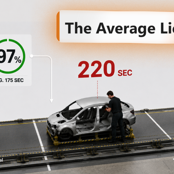
„With a cycle time of 180 seconds, variant A takes 130 seconds, variant B takes 175 seconds, and variant C takes 220 seconds. On average, the three options take about 175 seconds, which is below the cycle time. Variant A still results in 50 seconds of idle time, and Variant C exceeds the cycle time by 40 seconds. “


Idle times and time spread ratio are thus two sides of the same coin. The greater the time spread, the greater the tension between peak workloads and unused capacity. A single outlier can usually be accommodated through organizational measures. If such deviations occur regularly, the work distribution no longer matches the actual variant mix. This is precisely where line balancing comes into play.
Line Balancing for Stable Lines With a Fixed Cycle Time
Line balancing assigns tasks to workplaces on the line and determines which worker performs which tasks at which station. A task is the smallest meaningful unit of work that can be scheduled: a completed task with a planned standard time that specifies how long a worker needs to complete it. This standard time can be determined using established time-management methods; TAKTIQ supports MTM and MODAPTS, and will support REFA in the future.
Several tasks together form an order, that is, a single product to be manufactured in a quantity of 1. Depending on the model and variant, an order contains different tasks, the sum of which determines the assembly effort required for the product. In high-variety production lines, line balancing must therefore do more than simply distribute work evenly: it must take into account time spread, idle times, time spread ratio, and the frequency of individual variants.
An obvious solution is max line balancing. In this approach, the line is designed so that even the most time-consuming variant fits within the cycle. This provides reliability, but comes at the cost of idle time, since all the less time-consuming variants leave capacity unused.
Mixed line balancing, on the other hand, considers the actual distribution of work loads across the variant mix. Instead of designing each station for the worst-case scenario, it distributes the work loads in such a way that idle times are reduced and the time spread ratio remains manageable. What matters then is no longer whether a single variant temporarily exceeds capacity, but whether this load can be planned and managed within the overall system so that the line runs stably and efficiently given the actual order mix.
The transition from max line balancing to mixed line balancing is the key lever. It only becomes effective when combined with other mechanisms.
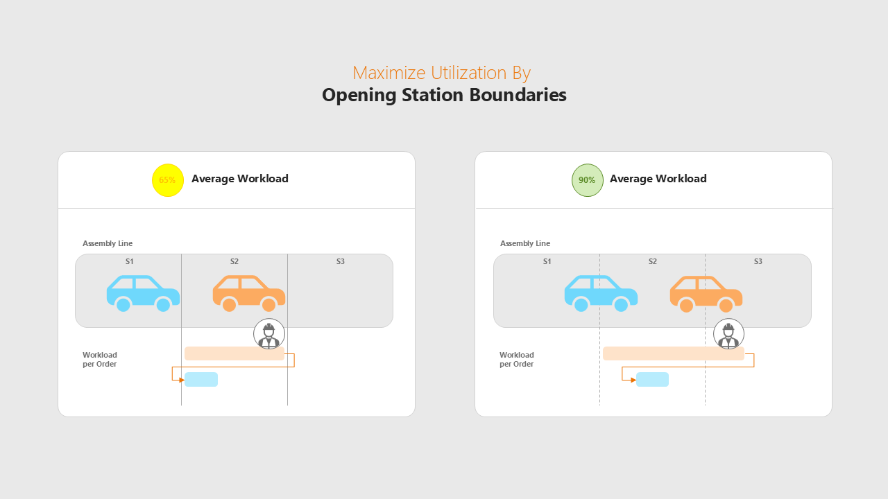
The first is intentionally limited drift. Drift occurs when a worker cannot complete an order entirely within the scheduled cycle time and finishes a part of the work in the following cycle. Station boundaries are not viewed as rigid in this context, but are controlled through a defined drift limit. This limit determines how far into the next station an order may be processed before planned drift turns into a drift limit violation. Drift is therefore not automatically a bad thing, nor is it synonymous with overload; rather, it is a planned tool for accommodating time-intensive variants, as long as it remains controlled and is balanced out over other cycles.
The second mechanism is sequencing. It determines the order in which products move through the line. If several complex variants follow one another in quick succession, this creates peaks in workload. If, on the other hand, variants with high and low labor content are strategically combined, the time spread can be reduced over the order sequence. Sequencing rules systematically limit such peaks: For example, they specify how often a complex variant may appear within a defined order sequence (density rules) or which variants should not follow one another directly (neighborhood rules). Our article on sequencing rules explains how these rules work in detail.
Another concept is the Vario Cycle. While the classic cycle is based on equal time intervals between products, the Vario Cycle uses variable cycle times: Products requiring more work are allotted more time, while those requiring less work are allotted correspondingly less. This relaxes the rigid output logic. Especially when a fixed cycle leads to excessive idle time, significant time spread ratio, or a constant need for support, the Vario cycle can be an interesting alternative, depending on the line’s logic.
Frequently Asked Questions About Production Planning
The cycle time is the specified timeframe within which a product must leave the line, calculated based on available production time and customer demand. The cycle time is the actual time required for a work cycle at a station and varies depending on the product variant, the worker, or material availability. The cycle time sets the framework; the cycle time shows the extent to which actual processing utilizes that framework.
Because products don’t move through the line as an average, but as specific orders in a specific sequence. A workplace can operate below capacity on average and still be regularly overloaded when several time-intensive variants are processed in succession. The key factor is time spread, that is, how much and how often the utilization fluctuates.
Time spread describes the extent to which workloads vary across the different variants. This refers to the overall distribution of times, including their values and frequencies, not just the range between the minimum and maximum. The greater the time spread, the greater the tension between idle time and the time spread ratio.
Max line balancing schedules the line based on the most time-intensive variant. This avoids time spread ratio but results in idle time for all less time-intensive variants. Mixed line balancing is based on the actual distribution within the variant mix and allocates work in such a way that idle times are reduced and the time spread ratio remains manageable, rather than designing each station for the worst-case scenario.
No, not necessarily. Drift occurs when a part of the work isn’t completed until the next cycle. As long as it remains within a defined drift limit and is offset by other cycles, drift is a planned tool for accommodating time-consuming variants. It only becomes critical when a drift limit violation occurs.


Bottlenecks Despite Line Balancing: Why Individual Workplacees Are Overloaded and How Line Balancing and Sequencing Work Together.
Learn More

Line Balancing in High-Variety Assembly: Why Manual Planning Has Its Limits and What Data-Driven Line Balancing Can Achieve.
Learn More
Why traditional lean tools reach their limits when there is a high degree of product variety, and why line balancing becomes the foundation for effective lean initiatives.
Learn More